How to Train an LLM: Part 1

How to Train an LLM by Omkaar Kamath

This is not a tutorial, it is my journey building a domain-specific model (domain under wraps till later blogs). In this blog (1 of N), I’ll set up basic pre-training infra, train a 1B Llama 3–style model on 8×H100s, and figure out how far that actually gets us.

While I have trained models in the past, none of them match the effort that I am about to put over the coming weeks. This blog was inspired by Nanochat and Olmo.

Why start with a good ol’ Llama 3–style config? Because I want a clean, boring baseline. Then we get weird or as some might say BLASphemous ;)

For data, I will use Karpathy's fine-web-edu-shuffled. Over the next few blogs, I want to improve my training infra, grow my own token farm - yes, we will engage in the art of token cultivation - and make architectural changes to make it inference-friendly according to the final capability I want these models to possess.

I want to support a 4096 context length but with the available compute and given attention is still painfully quadratic during training, it makes more sense to keep context shorter and increase batches. Generally, labs train on shorter context for 80-90% of the run and then, go ham in the last 10-20%, similar to Llama 3's schedule. Furthermore, in most web-scale datasets, most sequences are <2k tokens anyway, so generally, it's not like we have nice long samples to train on. Therefore, I will train on 2048 as my sequence length. I also omit cross-document masking for now.

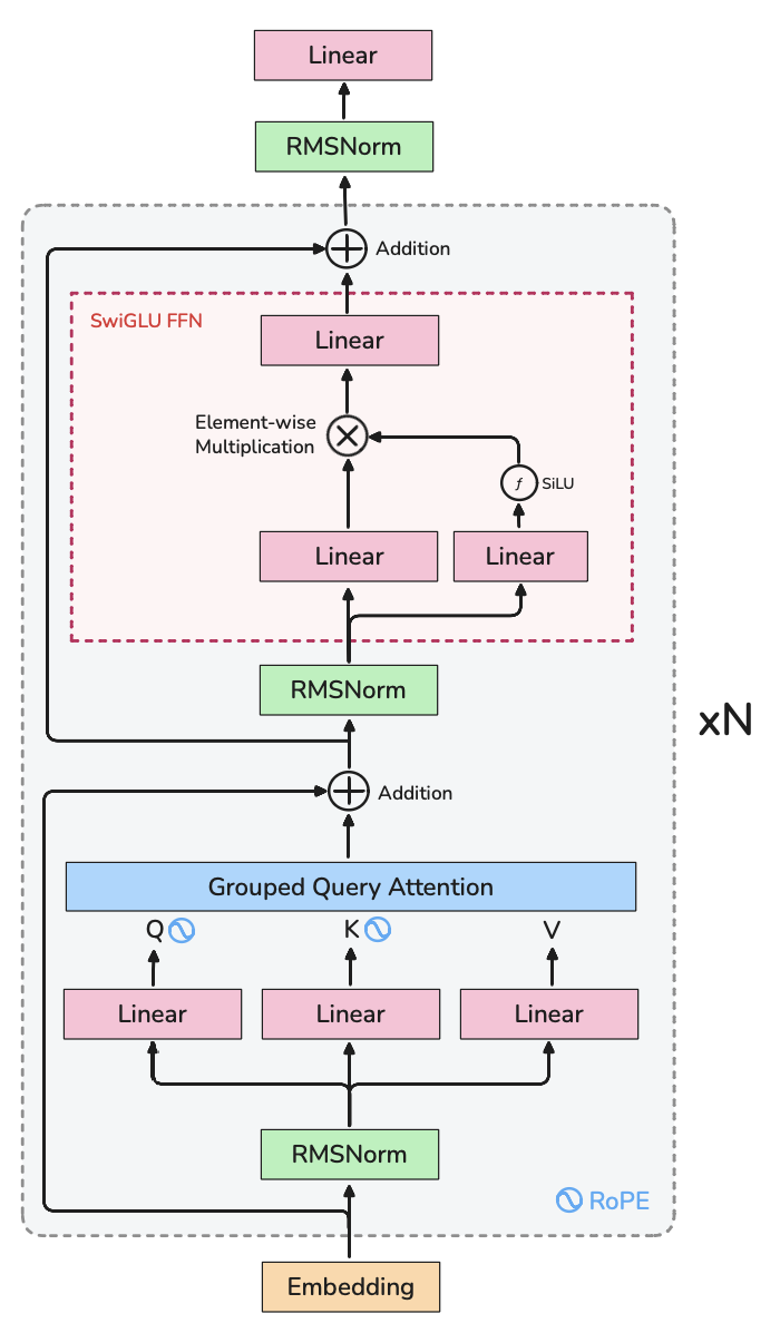
If you're not familiar with Llama-3's architecture, here's what we're working with: Llama 3 Architecture

This is the config I use for training:

@dataclass
class ModelConfig:
    rope_theta: int = 500_000
    vocab_size: int = 2**17
    hidden_size: int = 2048
    swiglu_hidden_multiplier: int = 4
    norm_eps: float = 1e-5
    num_attention_heads: int = 32
    num_hidden_layers: int = 16
    num_key_value_heads: int = 8
    tie_embeddings: bool = True
    attention_bias: bool = False
    mlp_bias: bool = False

A simple way to get model params in torch is sum(param.numel() for param in model.parameters()) = 1241581568 params (1.2B).

However, we can do this from scratch as well. Assuming group-query attention:

params = 
    vocab_size * hidden_dim 
    + n_layers * (
        hidden_dim + 
        2 * hidden_dim * hidden_dim + 
        2 * hidden_dim * hidden_dim / num_kv_heads + 
        hidden_dim + 3 * hidden_dim * intermediate_size
    ) + 
    hidden_dim +
    0 (<= tied embeddings)
= 1241581568 params.

Now, let's estimate memory usage, these are ballpark FP32 numbers to build intuition, not exact Nsight traces.

Total FP32 memory = (activations + weights + gradients + optimizer state) + misc.
Misc is for storing kernels, rope cache, etc. on the GPU, let's assign that 5GB.
Weights = 1241581568 params * 4 bytes / param = 4.97GB
Gradients = 1241581568 params * 4 bytes / param = 4.97GB
Activations = dependant on implementation. Let's say k * 1241581568, when batch size of inputs is [1, 2048]. On my experiment, on a non-compiled model, I get n around 1.6 and memory = 7.95GB. It scales linearly (I confirmed this empirically with an experiment) with batch size
Optimizer = first moment + second moment = 2 * 1241581568 = 9.94GB

However, one can't simply add these up to calculate peak memory as different stages retain and evict different tensors. This is the basic training process:

loss = model.forward(tokens[:, :-1], targets=tokens[:, 1:])
loss.backward()
optim.step()

In the forward pass, we use the inputs and weights to calculate activations. Peak Memory = Weights + Activations = (1 + 1.6 * n) * params.

During backwards, we use the activations and weights to calculate grads and then evict activations from memory. Peak Memory = Weights + Activations + Gradients = (2 + 1.6 * n) * params.

During the optimizer step, we use grads and optimizer state to update our weights and then free our grads. Peak Memory = Gradients + Optimizer State + Weights = 4 * params

One thing not accounted for above is the steady-state peak memory of the run. When we initialize the optimizer, it resides in our memory throughout the run. Therefore, for an [n, 2048] input, the backward step produces our memory peak which equals (4 + 1.6 * n) * params. When training with a batch size like n = 64, activation memory >>> then all other allocations combined!

Since torch's ops are not fused in eager mode, it saves each op's result as an intermediate activation for the backward pass, resulting in more memory reserved than needed. Thankfully, there is a known easy path to reducing activation memory, torch.compile, and a hard path for any unoptimized corner of the profile, custom CUDA kernels. Both try to fuse these ops which tries to eliminate intermediate activations!

Let’s talk about token budget (total tokens to train). Chinchilla scaling laws say a 1:20 ratio of params:tokens is optimal. I have 1B params, so 20B tokens is what I need to train on. My target batch size is 1M (2^20) tokens which I chose because GPT-3 XL was trained on 1M (2^20) batch size. 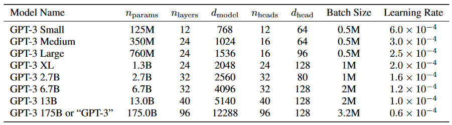GPT Params vs Batch Size Table

20B tokens / 1M tokens = 20000 training steps. Now, let’s do some back of the envelope math with the naive non-compiled numbers above, I have 8xH100’s meaning 80gb per gpu. Training through [1, 2048] tokens takes (1 + 1 + 2 + 1.6) * 1241581568 * 4 in FP32 memory which is 27.8GB of memory maximum. [N, 2048] tokens should take (4 + N * 1.6) * 1241581568 * 4 in FP32 memory which is 19.9GB + N * 7.95GB. On one 80GB H100 (accounting 5GB misc for kernels, etc), ~7 batches of 2048 tokens should fit given my optimistic, naïve calculations!

2^20 tokens (1,048,576) batch size is an input of shape [512, 2048] tokens. 8 GPUs doing [7, 2048] tokens at a time ([56, 2048] tokens being done at a time) means training one global batch needs to accumulate gradients over ceil(512/56) = 10 steps. Total steps needed to train the model is (20B / 1M) * 10 = 20000 * 10 = 200,000 steps

Remember this is without any optimizations. But, I have a few ideas up my sleeve which don't drastically affect accuracy: torch compile, flash-attn, gradient accumulation, mixed precision w/ BF16, etc.

Hitting a reproducibility snag

I calculated activation memory by measuring allocation on my Mac. When I ran these on 1xH100, the activation memory on a [1, 2048] tokens input is much higher. My mac shows 6.2GB while the H100 shows 22.5GB??

My first thought is could H100 have more intermediate ops which means more activations are saved? However, this does not make sense, ops are the same when not torch.compile'd. To debug this I referred to my confidants claude and chadgpt.

Claude was more helpful and was a better brainstorming partner. After brainstorming debugging ideas and spending time with my debugger to check theories off, we co-wrote a script to track memory layer-by-layer, and there lay the smoking gun: H100 attention activations per layer was OOMs (exaggeration to allow for funny pun) more compared to CPU attention activations. Upon deeper inspection turns out this was because CUDA SDPA with FP32 inputs falls back to naive attention (MATH backend) which materializes the full attention logit matrix. I confirmed this by manually casting QKV to bf16 and re-casting the output to fp32 to see the same activation memory allocation.

An idea here instead of manually casting dtypes on ops, it would be great to automatically lower the precision of select ops. This segues perfectly into our next section...

Optimization Time

In most LLM training runs, engineers have goals related to optimization: maximize MFU (mean flops utilization), maximize training throughput (tok/s), minimize communication overhead, etc. While we won't go too deep into them in this blog, we touch the basics.

Torch Compile

The first thing one should always try is running torch.compile(model). I wrote a very simple script for this section to test out optimization changes.

import time
import torch
from torch.optim.adamw import AdamW
from src.model import LLM
from src.utils import ModelConfig

device = torch.device('cuda')
config = ModelConfig()
model = LLM(config).to(device)
model.init_weights()
optimizer = AdamW(model.parameters())

for i in range(5):
    torch.cuda.reset_peak_memory_stats()
    start = time.perf_counter()

    tokens = torch.randint(0, 131072, (1, 2048), dtype=torch.int64).to(device)
    loss = model.forward(tokens, targets=tokens)
    loss.backward()
    optimizer.step()
    optimizer.zero_grad()

    torch.cuda.synchronize()
    end = time.perf_counter()

    print(f"Step #{i} | Time: {end - start:.3f} s | Allocated: {torch.cuda.memory_allocated() / 1e9:.2f} GB | Peak: {torch.cuda.max_memory_allocated() / 1e9:.2f} GB | Reserved: {torch.cuda.memory_reserved() / 1e9:.2f} GB")

Note: the huge time/peak in Step #0 & 1 is compilation + warmup. Use Step #2 onwards as steady-state.

Whatever my earlier math was on batch size was not accurate for unoptimized pytorch (likely underestimated misc. tensors). Without any optimizations, I can only fit [3, 2048] tokens as input without OOM'ing on the H100:

Step #0 | Time: 1.615 s | Allocated: 14.97 GB | Peak: 59.86 GB | Reserved: 61.05 GB
Step #1 | Time: 1.235 s | Allocated: 14.97 GB | Peak: 69.83 GB | Reserved: 72.32 GB
Step #2 | Time: 1.234 s | Allocated: 14.97 GB | Peak: 69.83 GB | Reserved: 72.32 GB
Step #3 | Time: 1.234 s | Allocated: 14.97 GB | Peak: 69.83 GB | Reserved: 72.32 GB
Step #4 | Time: 1.235 s | Allocated: 14.97 GB | Peak: 69.83 GB | Reserved: 72.32 GB

I tested the max input size with torch compile model = torch.compile(model, mode='reduce-overhead', fullgraph=True) and I can now do [4, 2048] inputs!

Step #0 | Time: 7.731 s | Allocated: 14.90 GB | Peak: 67.30 GB | Reserved: 82.94 GB
Step #1 | Time: 1.601 s | Allocated: 14.90 GB | Peak: 77.23 GB | Reserved: 82.94 GB
Step #2 | Time: 1.480 s | Allocated: 14.90 GB | Peak: 19.87 GB | Reserved: 82.94 GB
Step #3 | Time: 1.480 s | Allocated: 14.90 GB | Peak: 19.87 GB | Reserved: 82.94 GB
Step #4 | Time: 1.480 s | Allocated: 14.90 GB | Peak: 19.87 GB | Reserved: 82.94 GB

Let me explain briefly how torch.compile works. Normally, when running pytorch in eager mode (default) on a GPU, operations invoke a CUDA kernel, and there's overhead when invoking CUDA kernels one at a time. On a profiling chart, these look like empty spaces between each kernel running (referred to as "bubbles" shown below from PyTorch blog).

Bubbles in Torch Profile

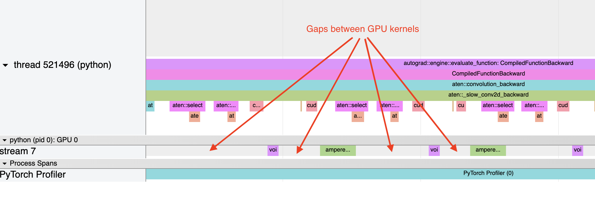
These bubbles reduce GPU utilization leading to a slower program. Torch compile tries to create a computational graph and fuse most of ops into bigger kernels to eliminate launch and memory-access overhead. With operations like for example, matmul -> element-wise op, torch.compile creates one kernel for matmul + element-wise which eliminates memory access overhead from element-wise.

The following image from the PyTorch Blog might help understand launch overhead minimization. CUDA Graph demonstration

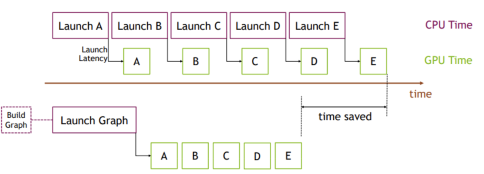
Torch compile uses Inductor as it's backend which generates Triton kernels, which means memory access patterns are also vastly improved and everything runs fast!

Mixed Precision

I haven't mastered the dark arts of low-precision training yet. H100's have support for fp8 but I will stick to bf16 mixed-precision for now. Explicit casting means setting the whole model to be the target type (bf16 in our case). BF16 has the same range but lower precision compared to fp32 which could lead to convergence issues due to rounding and small gradients being rounded to zero. Therefore, I keep weights and optimizer state in FP32, and wrap the forward in autocast so matmuls/attention run in BF16. That keeps numerical stability while storing many activations in BF16 (up to ~2× memory savings there).

Making this change is simple, I only have to add autocast to the forward pass:

with torch.autocast(device_type='cuda', dtype=torch.bfloat16):
    loss = model(tokens, targets=tokens)

The max input without OOM'ing is [16, 2048] which gets us the following result!

Step #0 | Time: 9.958 s | Allocated: 14.90 GB | Peak: 63.12 GB | Reserved: 78.59 GB
Step #1 | Time: 0.678 s | Allocated: 14.90 GB | Peak: 73.05 GB | Reserved: 78.59 GB
Step #2 | Time: 0.521 s | Allocated: 14.90 GB | Peak: 19.87 GB | Reserved: 78.59 GB
Step #3 | Time: 0.535 s | Allocated: 14.90 GB | Peak: 19.87 GB | Reserved: 78.59 GB
Step #4 | Time: 0.525 s | Allocated: 14.90 GB | Peak: 19.87 GB | Reserved: 78.59 GB

Fused AdamW

While I won't touch kernel land in this post, torch offers a fused AdamW which really saves on memory overhead.

It drops the last run's result by 5GB on the same [16, 2048] input tokens:

Step #0 | Time: 9.921 s | Allocated: 14.90 GB | Peak: 63.12 GB | Reserved: 73.63 GB
Step #1 | Time: 0.643 s | Allocated: 14.90 GB | Peak: 73.05 GB | Reserved: 73.63 GB
Step #2 | Time: 0.498 s | Allocated: 14.90 GB | Peak: 14.90 GB | Reserved: 73.63 GB
Step #3 | Time: 0.516 s | Allocated: 14.90 GB | Peak: 14.90 GB | Reserved: 73.63 GB
Step #4 | Time: 0.504 s | Allocated: 14.90 GB | Peak: 14.90 GB | Reserved: 73.63 GB

Gradient Checkpointing

We reduced activation memory by cutting some of it's size in bytes (fp32 -> bf16). Now, we will use gradient checkpointing which omits storing select activations during the forward pass and recalculates them during the backward pass as needed. This should let us really cut back on activation memory needed.

There is a good way and a lazy way to do this. Good way is to calculate memory and compute per op and evaluate the tradeoff + look at existing research. Lazy way is what I am about to do... which is brute force.

Let's add gradient checkpointing on every second layer with a [16, 2048] input, I get these results:

Step #0 | Time: 35.22 s | Allocated: 14.90 GB | Peak: 39.16 GB | Reserved: 49.72 GB
Step #1 | Time: 0.650 s | Allocated: 14.90 GB | Peak: 49.09 GB | Reserved: 49.73 GB
Step #2 | Time: 0.568 s | Allocated: 14.90 GB | Peak: 14.90 GB | Reserved: 49.73 GB
Step #3 | Time: 0.572 s | Allocated: 14.90 GB | Peak: 14.90 GB | Reserved: 49.73 GB
Step #4 | Time: 0.567 s | Allocated: 14.90 GB | Peak: 14.90 GB | Reserved: 49.73 GB

A 12% increase in compute time with a 24GB drop in reserved memory which is positively nuts.

What if we checkpoint all layers ... we get a 20% increase in compute time compared to no checkpointing for a 44GB drop in reserved memory.

Step #0 | Time: 36.29 s | Allocated: 14.90 GB | Peak: 19.87 GB | Reserved: 29.67 GB
Step #1 | Time: 0.640 s | Allocated: 14.90 GB | Peak: 29.03 GB | Reserved: 29.67 GB
Step #2 | Time: 0.603 s | Allocated: 14.90 GB | Peak: 14.90 GB | Reserved: 29.67 GB
Step #3 | Time: 0.593 s | Allocated: 14.90 GB | Peak: 14.90 GB | Reserved: 29.67 GB
Step #4 | Time: 0.600 s | Allocated: 14.90 GB | Peak: 14.90 GB | Reserved: 29.67 GB

Let's be cheeky and try [64, 2048] as inputs:

Step #0 | Time: 57.16 s | Allocated: 14.90 GB | Peak: 58.15 GB | Reserved: 73.76 GB
Step #1 | Time: 2.408 s | Allocated: 14.90 GB | Peak: 68.09 GB | Reserved: 73.77 GB
Step #2 | Time: 2.360 s | Allocated: 14.90 GB | Peak: 14.90 GB | Reserved: 73.77 GB
Step #3 | Time: 2.359 s | Allocated: 14.90 GB | Peak: 14.90 GB | Reserved: 73.77 GB
Step #4 | Time: 2.365 s | Allocated: 14.90 GB | Peak: 14.90 GB | Reserved: 73.77 GB

Could we do more?

I think this is perfect because I don't need gradient accumulation anymore. There might still be a few optimizations left on the table.

I tried switching to allowing the tf32 which takes fp32 inputs as we currently have it but performs GEMMs, by casting inputs to 19-bit floats (e8m10), on special tf32 compute units which should be faster. However, I did not notice any improvements in speed, so I omitted this. FYI, I simply added torch.set_float32_matmul_precision("high")... experts did I miss something?

Pytorch offers the Flash-Attention-2 (FA-2) backend which is fast but Flash Attention 3 is 50% faster on the H100 than FA-2. The only problem here is FA-3 needs to be compiled from source on my system and is known to take light years to compile. My process to get FA-3 is:

uv add packaging ninja
git clone https://github.com/Dao-AILab/flash-attention.git && cd flash-attention
cd hopper && python setup.py install
Use flash_attn_interface.flash_attn_func() instead of SDPA

Once FA-3 compiled, I tried it out in my code but I get an OOM. My FA-3 setup introduces a graph break in my LLM module which could add some inefficiency. I reduced batch size to 8 and noticed that it takes more time per step and memory than SDPA's FA-2 implementation. My conclusion is I messed up somewhere in my setup, something related to autocast, compile or checkpointing that probably does not gel well with FA-3. I will revisit this in my next blog and try to get it to work (it could be a big win).

I think checkpointing everything is not the best for my MFU, so I'd like to revisit my checkpointing scheme in the next blog as well. I can cut 34GB (64 * 2048 * 131072 * 2 bytes / param) by not materializing the logits before cross entropy loss, which will give me room to checkpoint less and increase throughput.

All the changes I have until now should not affect numerical stability and that is pretty important to preserve training convergence.

Since we plan to run distributed training, there is a question of communication overhead. GPUs need to sync gradients with each other after every backward pass. Given we only distribute bytes of our small model intra-node and intra-node bandwidth is pretty high, the overhead is a bit less relevant to us. In the next blog, I will showcase this more and look into overlapping so DDP will have minimal overhead. Another idea to minimize comm overhead is compressing + scaling gradients to fp16 which I'll bring into my next blog.

Data planning

Data planning is probably the most important part of the model training process. Garbage in, Garbage out.

I have two goals for the end model:

Mid-context length ready: 90% of the steps will have an input with sequence length 2048 tokens and the rest 4096 tokens.
Qualitative: Good at english, math and code tasks for a particular downstream task.

Given that our scope is to start off simple, I want to ensure my codebase works and run converges first and so, I will simply train on Karpathy's fine-web-edu-shuffle.

General training infra

I'll run through this section as it's the finer more boring details.

Checkpointing

Fairly straightforward, I used torch's save and load APIs to save:

checkpoint = {
    "model_state_dict": model.state_dict(),
    "optimizer_state_dict": optimizer.state_dict(),
    "scheduler_state_dict": scheduler.state_dict(),
    "dataset_state_dict": dataset.state_dict(),

    "python_rng_state": random.getstate(),
    "numpy_rng_state": np.random.get_state(),
    "torch_rng_state": torch.get_rng_state(),
    "cuda_rng_state": torch.cuda.get_rng_state_all() if torch.cuda.is_available() else None,
    
    "step": step,
    "best_val_loss": best_val_loss,
    "model_config": asdict(model_config),
    "train_config": asdict(train_config),

    "versions": {
        "torch": torch.__version__,
        "cuda": torch.version.cuda if torch.cuda.is_available() else None,
        "python": sys.version,
    },
}

Checkpointing needs GPU-CPU sync of weights and all kinds of state which is pretty heavy and stalls the whole run. To minimize checkpointing, I checkpoint every 2500 steps and on the last step for now. Industry also has checkpointing every time validation loss goes down. There are smarter ways to checkpoint (async) and I might get into it if I see run performance taking a big hit.

Weight Initialization

I'll be honest I have no prior experience initializing weights for a model of this size. I looked through literature and Nanochat and ended up getting Deep Research to check out papers to suggest ideas. I ended up doing this:

def init_weights(self):
    self.apply(self._init_weights)   
    n_layers = self.config.num_hidden_layers
    for block in self.layers:
        std = (self.config.hidden_size ** -0.5) / (2 * n_layers) ** 0.5
        torch.nn.init.normal_(block.attention.o_proj.weight, mean=0.0, std=std)
        torch.nn.init.normal_(block.swiglu.down_proj.weight, mean=0.0, std=std)

def _init_weights(self, module):
    if isinstance(module, nn.Linear):
        std = 1.0 / module.weight.size(1) ** 0.5  # 1/sqrt(fan_in)
        torch.nn.init.normal_(module.weight, mean=0.0, std=std)
        if module.bias is not None:
            torch.nn.init.zeros_(module.bias)
    elif isinstance(module, nn.Embedding):
        torch.nn.init.normal_(module.weight, mean=0.0, std=0.02)

Learning rate schedules

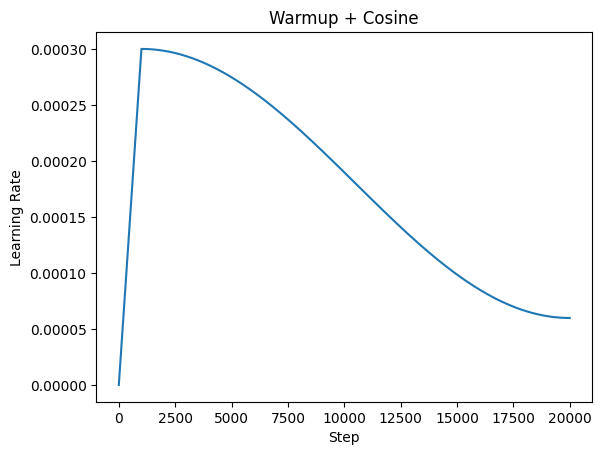
I have consumed enough content to know to use a linear warmup till m steps and then use a cosine schedule:

scheduler = get_cosine_schedule_with_warmup(
    optimizer,
    warmup_ratio=train_config.warmup_ratio,
    num_training_steps=train_config.num_iterations,
    min_lr_ratio=train_config.min_lr_ratio,
)

It looks like the follows: LR schedule: Warmup + Cosine

Battling the training overlords

I expected to face some turbulence during training. I have read multiple great blogs about training convergence issues like the famous Marin 32B's loss spikes blog. I do think convergence issues are more common in larger training runs, so hopefully we do not run into them.

Because training on 8xH100's directly without verifying every line of code works is a catastrophic waste of money, I rolled out this run in 4 stages. First stage is local device testing where I ran training on my Macbook on a much smaller model. This was to identify any general pytorch related bugs that I might have introduced.

Once I solved those, I ran it on 1xH100 where I squashed a few minor torch.distributed cleanups and cuda-related errors. I noticed over 250 steps that my loss was down and to the right which is a good sign. The loss starts off as ~12. Since the model has random weights and no knowledge at the beginning, the probability of getting any token is 1/vocab_size and therefore, cross entropy loss is -ln(1/131072) = 11.78, so we are bang on the expected first loss value.

With [64, 2048] inputs on the 1xH100 and over 256 steps, the model went from a loss of 12.26 to 6.18. To get a better idea of how my actual training run will do, I set grad_accum_steps to 8 (effective batch size = [512, 2048] tokens) which is effectively the batch size of my actual training.

Then, I hit a snag. Torch.compile + gradient accumulation has some quirks, since I run backward() without runnning the optimizer each step, I get Error: accessing tensor output of CUDAGraphs that has been overwritten by a subsequent run. I spent a bunch of time trying different things like the suggested torch.compiler.cudagraph_mark_step_begin et al to no avail. Finally, an idea was to disable CUDA graphs all together (maybe bad idea in the long term?) and use the 'default' torch.compile mode and it worked! Now, my problem is with higher batch sizes, reserved memory explodes (reduce-overhead mode was saving me all this time). You know what, I don't even need grad accum for now so this is not a pressing problem, let's move on to 2xH100 with the proper torch compile and no grad accum.

I wanted to run this on a 2xH100 to minimize costs if I end up hitting a snag and debugging, while still checking for correctness on a distributed setup. My first mistake with this run was guessing the order of applying ddp and compile, note: always apply model = DDP(model, ...) first and then model = torch.compile(model, ...). Ok, so are we finally sorted? Nah, the run failed again because of another CUDA-graph related problem. I decided to try and relax the graph constraint by turning fullgraph=False and it worked! If that did not work, I would have made torch compile mode='default' again but the run and I really don't enjoy the increase in reserved memory (and subsequent OOMs) it causes. FYI, I use torchrun for easy distributed training.

Finally, it was time to run on the 8xH100 cluster. It works from the get-go!

A problem I had was around 15k steps my loss was stagnant. My intuition was that the learning rate is too low, there was no way for me to verify this given I was not logging things like ||update|| / ||param|| which would have helped me debug this more. So, I decided to stop training, load back the 15k checkpoint with a different scheduler (0.5*base_lr, very low warmup steps, higher minimum lr ratio) for 5000 steps. To no avail, I could not revive the run, so I decided to save some money, stop the run and leave the checkpoint as is at 15k steps.

Doing this motion allowed me to verify me checkpointing logic (although I should have tested it on 1xH100 first) and fix all the minor bugs. Major bugs mean all the 10+ hours of 8xH100 money is wasted. I don't enjoy YOLO runs and this one did not work.

This is my graph for the first 15,000 steps:

15k steps of training a 1B model

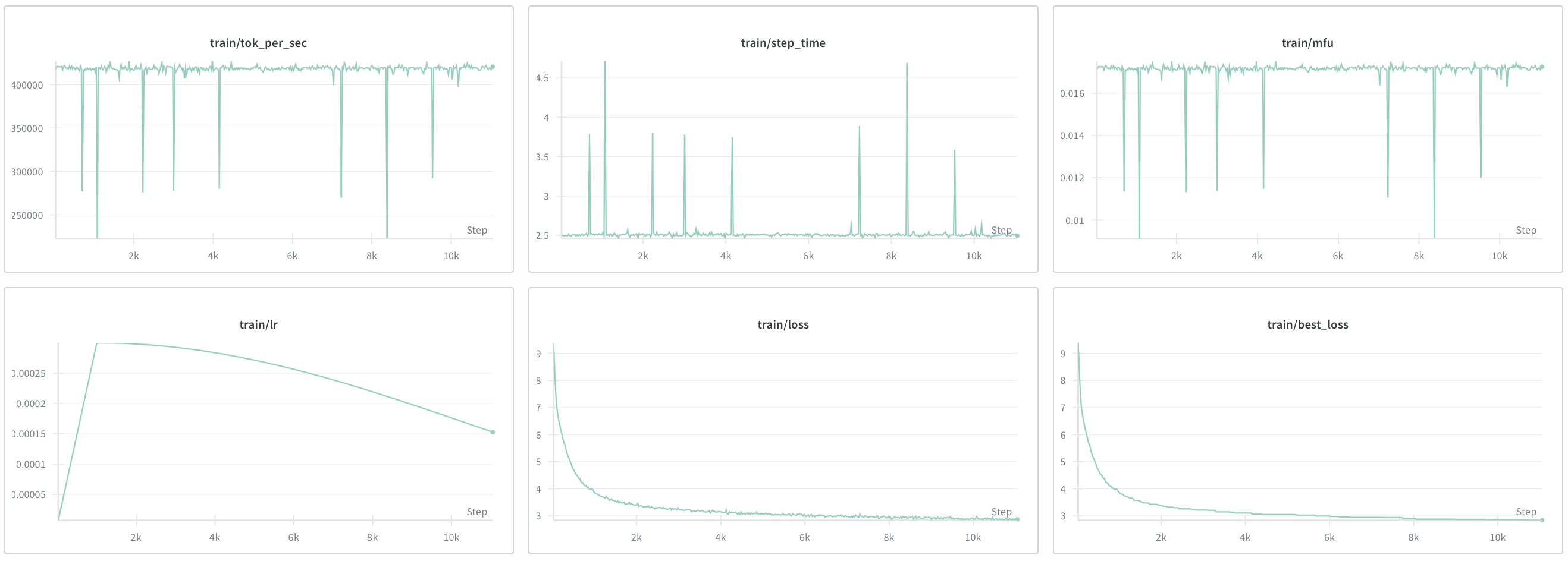
Overall, this was fun, however my MFU is at 18% & train throughput was at 400k tok/s which is no bueno. Running checkpointing on every layer impacted throughput a lot, however it allows me to skip gradient accumulation, so I need to consider this tradeoff in my next article.

Given future roadmap and the need to train more models, I want to minimize costs and inefficiency as much as possible while making my performance gains translatable to all types of models / runs. These gains will come over the next post and will be easy to test now that we have a stable, working V0 training infra.

Reflections

I have a few reflections. I started off with a massive scope but realized it's too much for a fresh codebase. I wrote this messy but working first iteration, then refined it over the course which reminds me of this picture: SpaceX's thruster optimization

It's much easier to iterate from bad to good than end up at good straight away. Don't get me wrong my repo is still far from SOTA but it provides a clear working implementation which I can abstract further later. That brings us to my second reflection, I had to rely on others' observations for learning rate, weight inits, scheduler and other hyperparams. Great researchers have a mix of empirical evidence along with mathematical intuition for what works based on 100s of past runs. It's something that I'll just have to iterate and read more papers on.

Extras

Tim Dettmers has a library called bitsandbytes which is widely used for quantization. Check this paper to learn more. Anyway, they have an AdamW8bit optimizer which is commonly used in finetuning.

If pre-training with this over 8k+ steps converges, I can basically get away with using this 8bit version! So I brought it into my 1xH100 training run along with StableEmbedding which is the recommended setting. My reserved memory dropped by 10GB and these are my wandb runs 8bit vs fp32 AdamW: NF4 vs FP32 AdamW

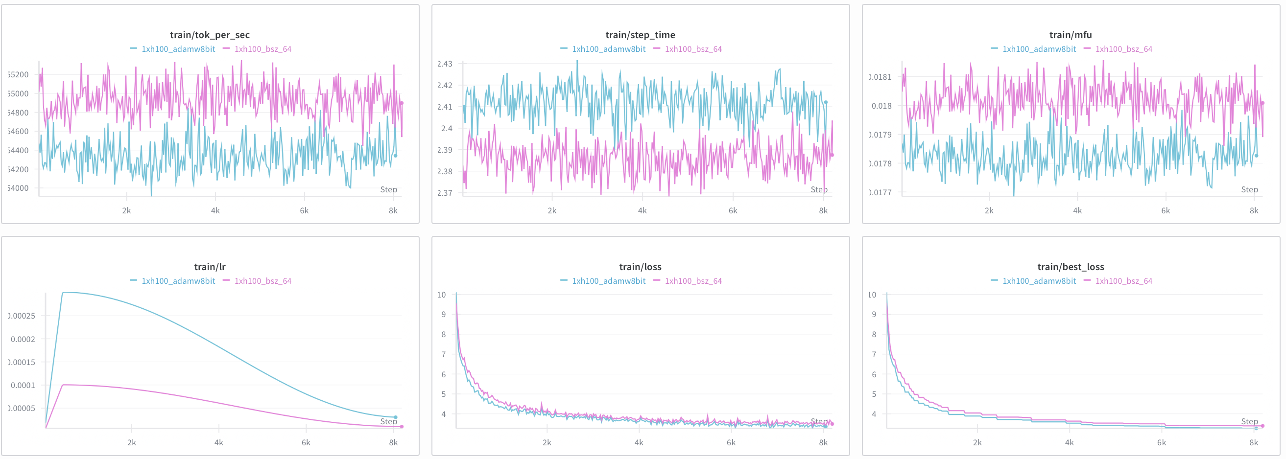
At first glance, it seems like it converged even better than the fp32 variant. However, upon looking carefully, you might notice my blunder. I messed up and gave 8bit AdamW 3x the peak learning rate. Would I scrap all my results though? No, while AdamW8bit > AdamW32bit is inconclusive, AdamW8bit looks stable enough. I am planning to use it in my next run as it reduces memory while still converging.