Pipeline Parallelism

I am trying to get better at Pytorch's dist API and decided to implement all forms of parallelism from scratch with torch.dist (I'll write about this some other time). The others were fine, but something about pipeline parallelism (PP) really entranced me.

This blog by Simon is a fantastic intro to pipeline parallelism. I'd recommend giving it a quick read before proceeding.

There is a certain beauty in old and new PP schedules, and I wanted to share that with this world in this blog. It's also surprisingly therapeutic and fun to draw out pipeline algos in google sheets.

Basics

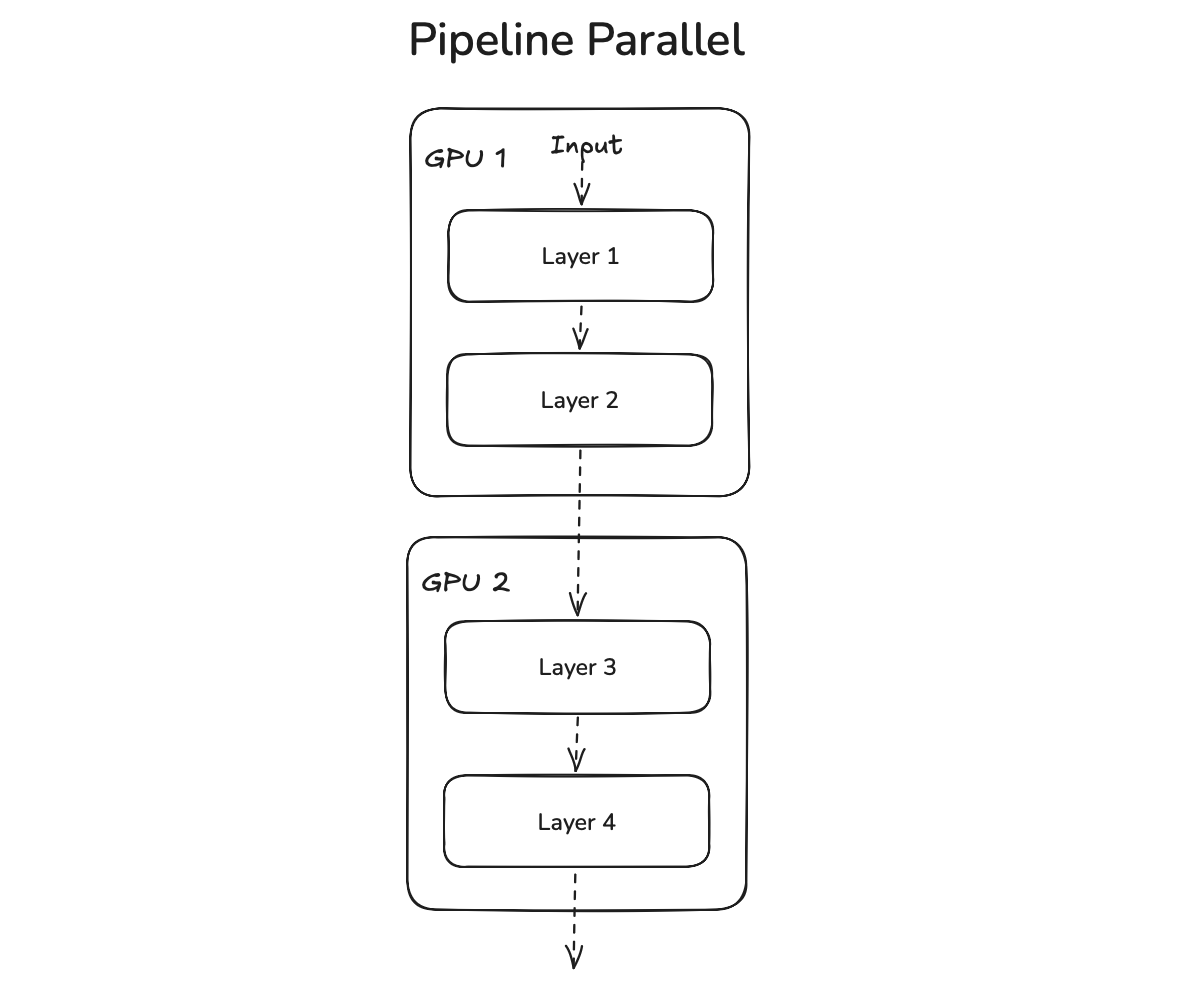
Read Simon's blog, but if you are in a crunch, PP's goal is to chop the large model into stages (or sets of continuous layers) and distribute them across ranks like so:

Notation

For each scheme, I'll cover the bubble rate, peak memory and communication costs in terms of these variables:

p = Pipeline stages (number of cuts on the model)
m = # of Microbatches (number of cuts on one batch)
v = # of stages per device
t_f, t_b = Time for forward and backward pass on one stage
M = Activation memory stashed on one microbatch on one stage
a = Size of activation tensor in forward (and same size gradient tensor in backward)

Bubble rate measures the fraction of time compute does no work. It is a good indicator of how much of a cluster's time will be wasted.

Schemes

This seems like such a simple concept, but in practice there is a lot more than meets the eye. PP researchers' goal is to come up with better schedules that reduce memory requirements, bubbles (we'll cover this in a bit), find ways to accommodate checkpointing, and much more. A schedule is simply the order and type of work running on each rank over time. The underlying PP abstraction writes a state machine which reads this schedule and executes.

Naive

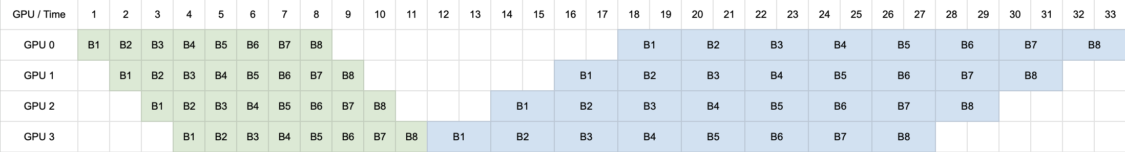
Look at this Naive schedule:

Green denotes forward pass and blue denotes backward pass.

A forwards pass of a linear layer is one matmul, while the backwards pass is two (one to calculate weights and one to calculate input's grad), which is why the backwards pass is shown as twice as long as the forwards.

4 GPUs, 1 batch. It's running a full batch on each layer and forwarding the activations to the next layer. Final layer calculates loss and runs backward, then sends its input gradient (the gradient w.r.t. the previous stage's output) to the previous layer which runs backward on it and so on.

There are a few key assumptions here. Communication costs are assumed to be negligible. It's not only too much work in Excel to resize cells to show it, but it's also a headache to account for when making these algos.

Communication volume = 2(p - 1) * m * a

Peak memory = m * M

Bubble rate = (p - 1) / p

GPipe

Some people noticed splitting the batch into micro-batches can yield an almost linear speedup, called it GPipe and wrote a paper on it. GPipe schedule

Your receiving GPU does not need to wait for the full batch's forward or backward to complete, only the microbatch's.

Let's talk about bubbles and why GPipe is better. Look at the Naive schedule again, notice how much whitespace there is. A unit of whitespace or unit of time where a GPU is not doing any work is a bubble. These are pretty expensive at scale since one pays for the GPU regardless of whether it's doing work or not.

Majority of Naive schedule is made up of white squares so I won't even bother counting it. GPipe gets more useful work done in less time by overlapping a lot of the compute.

Communication volume = 2(p − 1) * m * a

Peak memory = m * M

Bubble rate = (p-1) * (t_f + t_b) / ((m+p-1) * t_f + (m+p-1) * t_b) = (p-1) / (m+p-1)

There is however one problem with GPipe...

1F1B

The 1F1B schedule can solve that problem with GPipe.

If you look at GPipe carefully, notice how before the first backward pass can start, it needs to store all 8 microbatches' activations, which leads to high peak memory usage. The activation only needs to be stashed until that stage's backwards is done, after which it can be deleted (which reduces memory).

Now look at 1F1B's schedule: 1F1B schedule

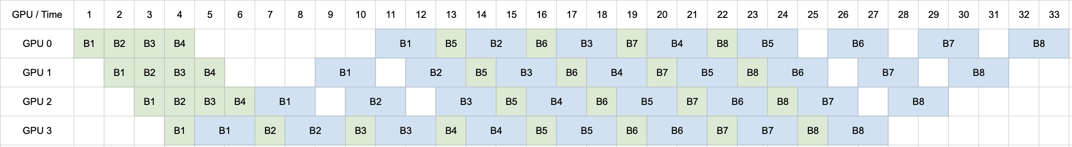
Instead of working with all 8 microbatches at a time, we first forward through the first 4 microbatches and then strictly alternate one-forward-one-backward. While the number of bubbles is the same as GPipe, peak memory drops as we delete activations once that microbatch's backwards is done.

Communication volume = 2(p − 1) * m * a

Peak memory = p * M

Bubble rate = Same as GPipe = (p-1) / (m+p-1)

Interleaved 1F1B

The Interleaved 1F1B schedule goes one step further and pushes for slimmer stages. So instead of 1 stage being 4 sequential layers, 1 stage is now 2 sequential layers and 2 stages are stored on one rank instead.

Given 4 GPUs and 8 sequential layers, GPU 0 will get layers 0 and 4, GPU 1 will get layers 1 and 5, and so on. This is the schedule: Interleaved-1F1B schedule

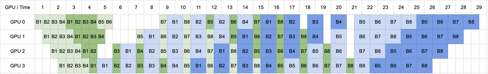
The early (0-3) layers are shown with lighter shades and later (4-7) layers with darker shades.

Because each stage is divided half (relative to simple 1F1B), for diagrammatic consistency, each time unit is divided in half, and therefore each white space is 0.5 bubbles. There are 36 white spaces which means only 18 bubble units (compared to regular 1F1B). Instead of completing in 33 units of time, it completes in 28.5!

Communication volume = 2(v*p − 1) * m * a

Peak memory = p * M

Bubble rate = (p−1) / (vm+p−1)

Zero Bubble PP

Sea AI Lab's ZBPP paper then introduced a zero bubble (in steady state) schedule. I am showing the ZB-H2 variant's schedule here: ZB-H2 schedule

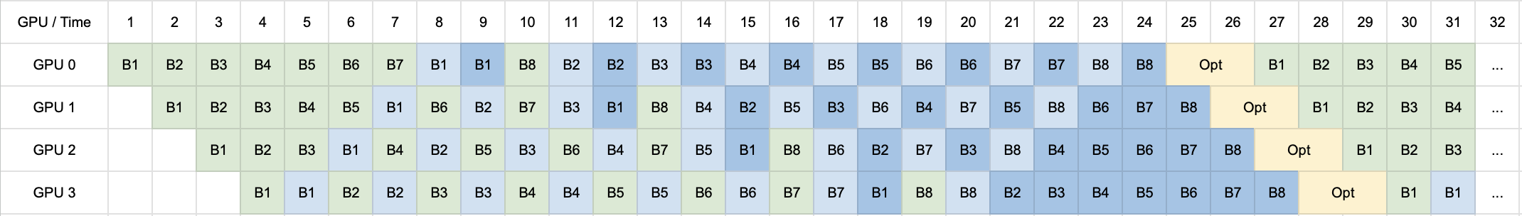
This schedule splits up the two matmuls of the backward pass shown above as the light blue square (which calculates input grad) and dark blue square (which calculates the stage's weight grad).

The previous layer only needs the input grads during the backwards pass (blocks previous stage) while the weight grads are only needed right before the optimizer run (to actually train the model).

In yellow is the optimizer step, the assumption is it takes up as much time as the full backward pass.

This one is handcrafted which is impressive, they figured out a way to pipeline the optimizer state to eliminate bubbles in subsequent epochs. Just keep in mind, these are ideal condition schedules which do not always reflect real conditions.

Communication volume = 2(p - 1) * m * a

Peak memory = Way more than 1F1B

Bubble rate = 0 (in steady state)

Note on Others

There are many other important / interesting schedules, some notable ones from what I have seen are Chimera (bi-directional pipelining), BitPipe (more bi-direction), Deepseek's DualPipe (bi-direction + work splitting + interesting schedule specifically for cross-node expert parallel) and more. I simply wanted to cover the main classes of these schedules.

PipeDream was actually meant for async pp, I did not cover this because 1. it is a bit hard to understand and 2. it fell out of favor for synchronous training because weight staleness hurts convergence.

Conclusion

What I learned from all this is the standard tools in your shed should be micro-batching (to reduce bubbles), work-splitting (to allow for better comms / computation overlap), interleaving (multiple stages per device), bi-direction and building hand-crafted schedules for target workloads.

All this gave me the idea of formulating a MILP problem to minimize bubbles in a schedule, I was happy to see research on this already exists (Zero Bubble Pipeline Parallelism paper has it). The Real World™ doesn't have 1:2 for F:B passes, calculating forward vs backward time per stage and getting a solver to build a case-specific perfect schedule is a great idea.

As long as you have a state machine type runner to orchestrate schedule running, running any verified schedule should be easy. Also note that the above schedules are shown for 4 ranks, other microbatch and ranks need other schedules.

I plan to come back and add ideas to this blog if I come across any other cool schedules.