The Illustrated FastVLM: Apple
Apple's FastVLM is underhyped. It's a family of small models that pack a punch in terms of capability for their size. This project came to be because I wanted to dive deeper into VLMs. Walkthrough my code (adapted from the paper) along with this article for better understanding.
In today’s AI race, frontier models are often trained at massive costs and then open-sourced. By distilling larger models into smaller efficient architectures, you get cheap, high-quality models that run seamlessly on target hardware. This approach offloads the costly task of training huge teacher models, and makes it cheap to produce student models that are easier-to-align, faster, and hardware-friendly. By owning the hardware stack, Apple's incentive with this research is not only to ship better models, but also to guide future chip and software co-design.
This topic is susceptible to exploding in complexity, so I tightly limit scope to the architecture of the inference-time model and why this model is so efficient while foregoing details like training the model itself.
FastVLM
FYI a VLM = vision encoder -> projector -> LLM. ViT is the encoder backbone that takes an input image, runs preprocessing (will talk about this later), then forwards it through a deep network and finally, outputs one embedding per image token. These embeddings are to be concatenated with the language model's embedded input and ran through an LLM like in usual auto-regressive text gen.
Checkout the following top-level architecture from Apple's FastVLM paper showcasing the architecture.
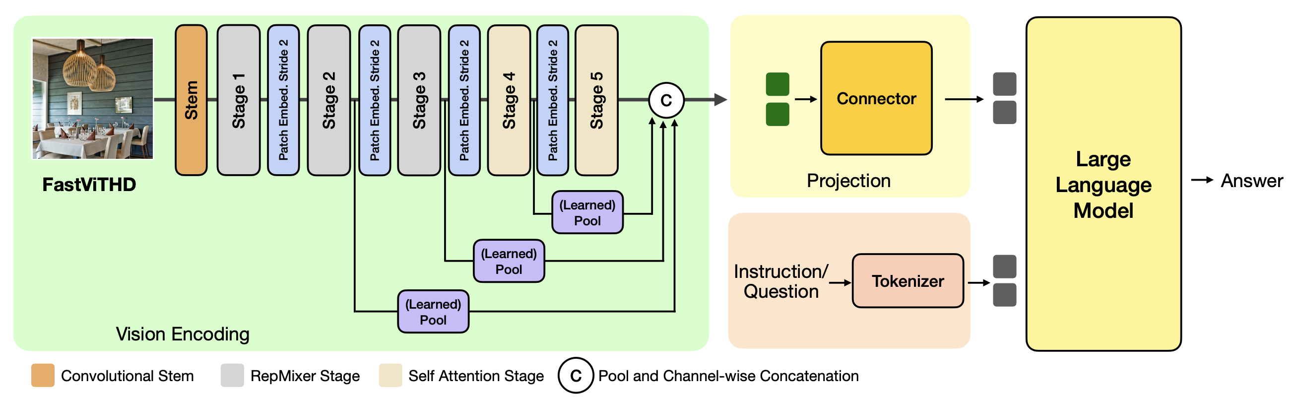
My code has been segmented in the same sections as the image above which should make it easier to follow.
Vision Encoder
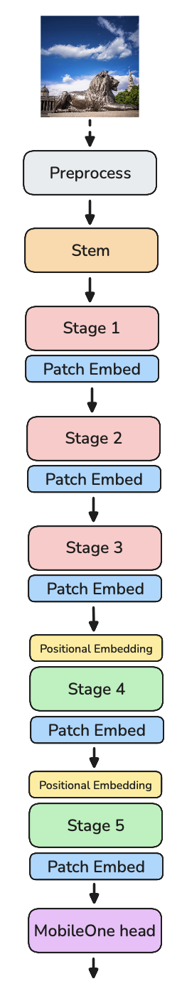
The vision encoder can be broken up into a few repeated blocks. Different colors in the ViT architecture below represent different blocks.
Preprocessing
Preprocessing is simple, standardization across channel and cropping the image to (1024, 1024). The following code comes from my implementation.
image = Image.open('./image.jpg').convert("RGB")

img_tensor = torch.tensor(CLIPImageProcessor(
    crop_size={"height": 1024, "width": 1024},
    image_mean=[0.0, 0.0, 0.0],
    image_std=[1.0, 1.0, 1.0],
    size={"shortest_edge": 1024},
    return_tensors='pt'
)(image)['pixel_values'])
Different ViTs handle high resolution differently. Some just patchify (split into fixed chunks), while others like FastViT-HD use a learned tokenizer (convs at the stem) to compress resolution while expanding channels.
Stem
The stem = 3×3 Conv + GeLU + 3×3 Depth-wise Conv + 1×1 Conv
Together, they shrink resolution and boost channels: [3, 1024, 1024] --> [96, 256, 256].
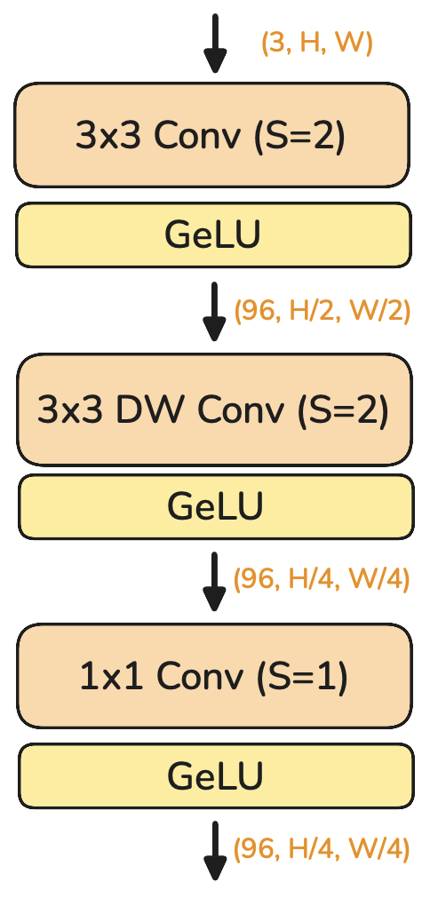
Depth-wise convolutions + point-wise (1x1) convolutions are 5-10x more efficient than a standard convolution with the same kernel size. Think of the stem as a smart tokenizer.
Stage 1-5
The five stages after stem all look similar:
- Each has N blocks, each with:
- one TokenMixer (either conv-based or attention-based)
- one ConvFFN (the MLP part)
- Each has a Patch Embed (downsampling)
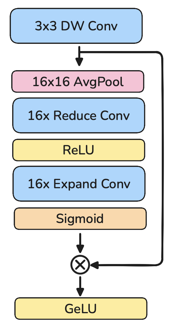
The 5 stages after stem are similar. Every stage has one Patch Embed and N blocks containing one TokenMixer (explained later) and one ConvFFN. In the first three stages, the TokenMixer is a 3×3 depth-wise conv (based on RepMixer). In stages 4–5, it switches to self-attention (after more downsampling). Structurally, this mirrors a transformer block: attention + MLP. Notice how TokenMixer + ConvFFN is structurally similar to the transformer decoder block (Attention + FFN).
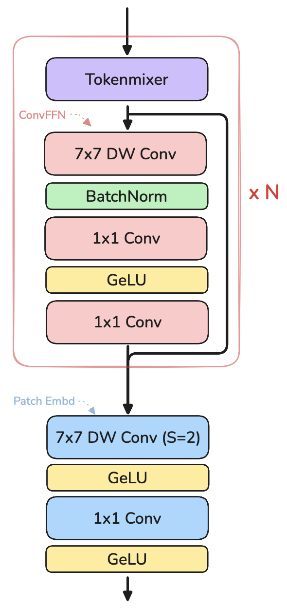
The above is how one stage looks like. Stage 5 does not have a PatchEmbed layer.
Note: before stages 4 and 5, they introduce conditional positional embedding layer (7×7 depth-wise conv) to inject position information.
> Receptive field and Token mixers
A receptive field is how much of the original image a feature can see. Therefore, convolutions inherently have local receptive fields (as big as the conv kernel) while self-attention (with no mask) is global. Because self-attention is an expensive operation, paper chooses to run the cheaper convolution token-mixer and downsample for the first three layers. Then, once the representation has been downsampled enough (8x in this case, [96, 256, 256] --> [768, 32, 32]), it uses attention as a token mixture to increase receptive field while keeping compute overhead low.
ViT head
After the 5 stages, the encoder has a head that pools multi-scale features into final per-token embeddings the projector will consume.
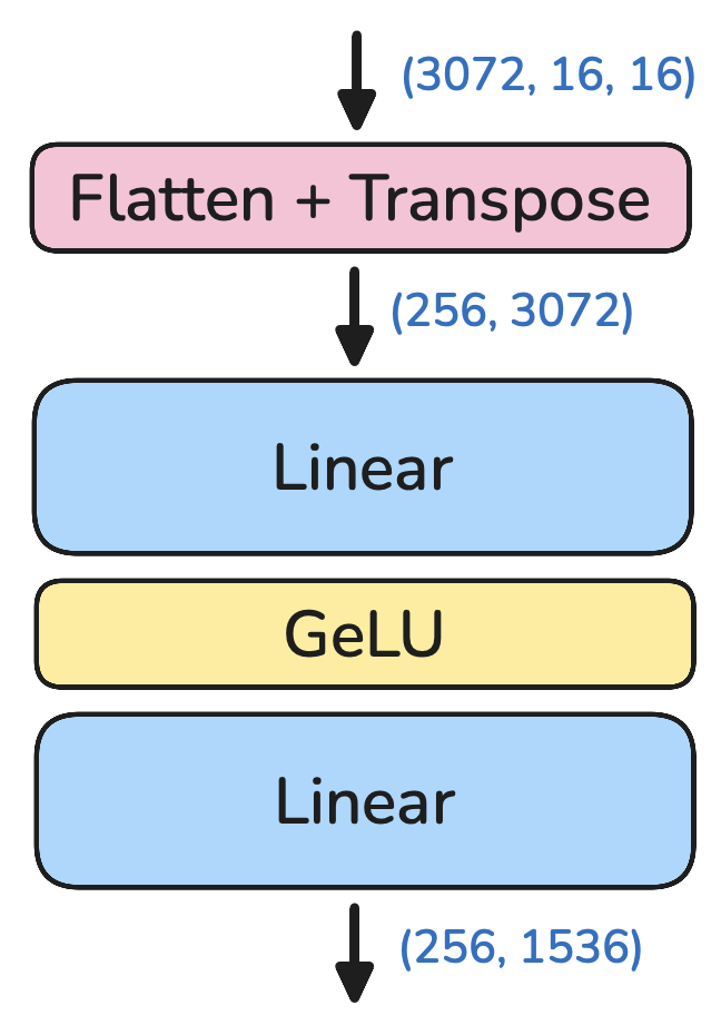
Projector
Think of the projection (or “connector”) layer as a translator between the ViT’s embedding space and the LLM’s embedding space. This is a simple MLP, but surprisingly powerful: train just this connector well and you can get a vision encoder to play nicely with any LLM.
LLM
This part is a standard LLM. Before tokenization, we look for <image> in the prompt, tokenize and embed everything before and after, then add the image embeddings in between, and finally pass it through the LLM as is normally done in auto-regressive text gen.
Where does the efficiency come from?
The goal of this paper was not to just be efficient, they wanted to allow efficient processing of high resolution (1024x1024) images.
Given FastViT-HD produces >4x fewer tokens for a high-resolution image compared to other ViTs, LLM prefill time is relatively much lower.
Performing convolutions early for token-mixing and attention when representation is smaller cuts compute while upholding quality.
The convolution paths (stem, patch-embed, ConvFFN, RepMixer) use batchnorm which can be fused into a single convolution at inference. However, batchnorm might not generalize too well on out-of-distribution data.
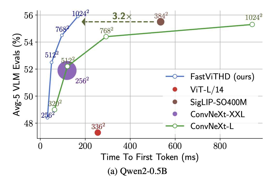
As shown in the above graph from the FastVLM paper, for 1024x1024 resolution, FastVIT-HD has fast TTFT and performs well on evals.
P.S.
Some out of scope points I wanted to mention:
- The architecture of the train-time and inference-time model is different. They make use of over-parameterization and then fold identities and multiple convolutions into one convolution during inference time. It's in the FastViT paper. I am writing an explanation for this next.
- Training the model follows the same 2-stage training pipeline from LLaVA-1.5. During the first stage, only the projector is trained. In the second stage, they run SFT on the vision encoder, projector and the LLM.
By Omkaar Kamath