Distributed training LLMs from 1st principles

Fun story: When I was in 3rd year uni, I was training a model on my M1 mac for a project, but it was too slow. So, I figured what if we train the same model (same weights w/ same seed) on two separate macs w/ two different data splits, half the steps and then average the weights. I stayed up all night implementing it and the resulting model was a bit better. I looked into this more and my idea was a very dumb version of something called "distributed training". I later built a simple distributed training module: github, video.

While the concepts are simple, there is a lot going on behind the scenes of large model training / inference. I wanted to write this post / worklog and run some fun simulations to figure out the best configurations.

ML uses complicated terms and jargon to gatekeep these ideas for whatever reason. I hope you come out of this with a solid intuition, the terms itself are not too important.

Lastly, to really understand something, you must implement it from scratch. I could have used torchrun + torch's dist module but I wanted to be as close to the base of the abstraction pancake stack.

Edit: I end up early concluding this blog because I realized it's redundant and there are better resources out there that go in more detail.

Communication collectives

There are a limited number of ways to send data between compute devices (e.g. GPUs), these are called communication collectives.

These diagrams are remixed from NCCL's official page.

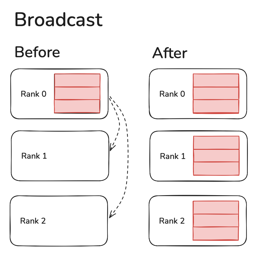
Broadcast

Broadcast simply sends data from current device to all other devices.

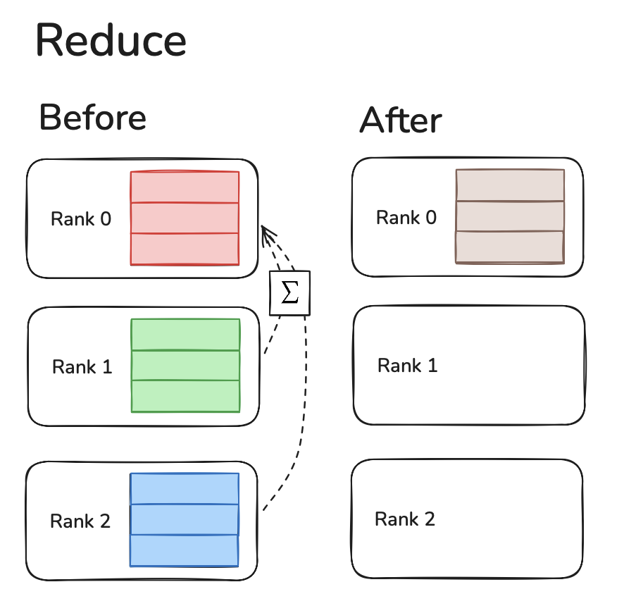
Reduce

Reduce is where data from all devices are received on one device and ran through a reduction operation (like SUM, MIN, MAX).

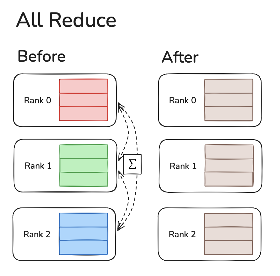
All-Reduce

All Reduce is similar to reduce but all the devices get the same reduced data.

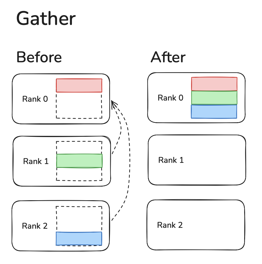
Gather

Gather gets pieces of data from other devices and stores a stacked copy of all the data.

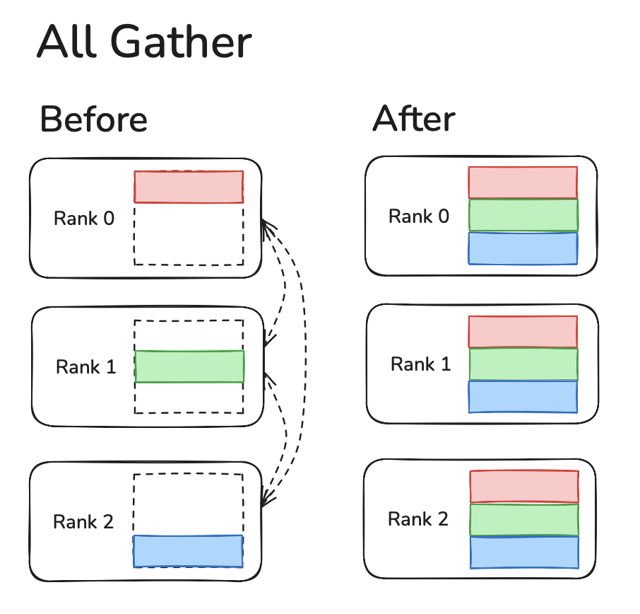
All-Gather

All Reduce is where data from each device sends all other devices it's data and runs an operation (like SUM, MIN, MAX) to reduce the data.

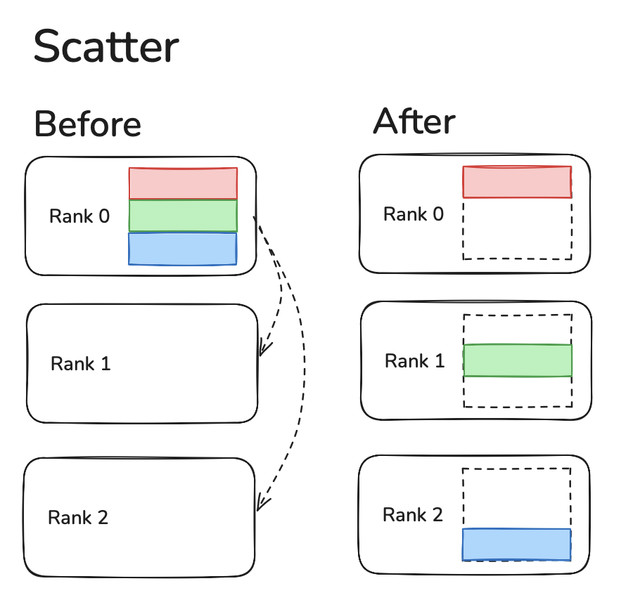
Scatter

All Reduce is where data from each device sends all other devices it's data and runs an operation (like SUM, MIN, MAX) to reduce the data.

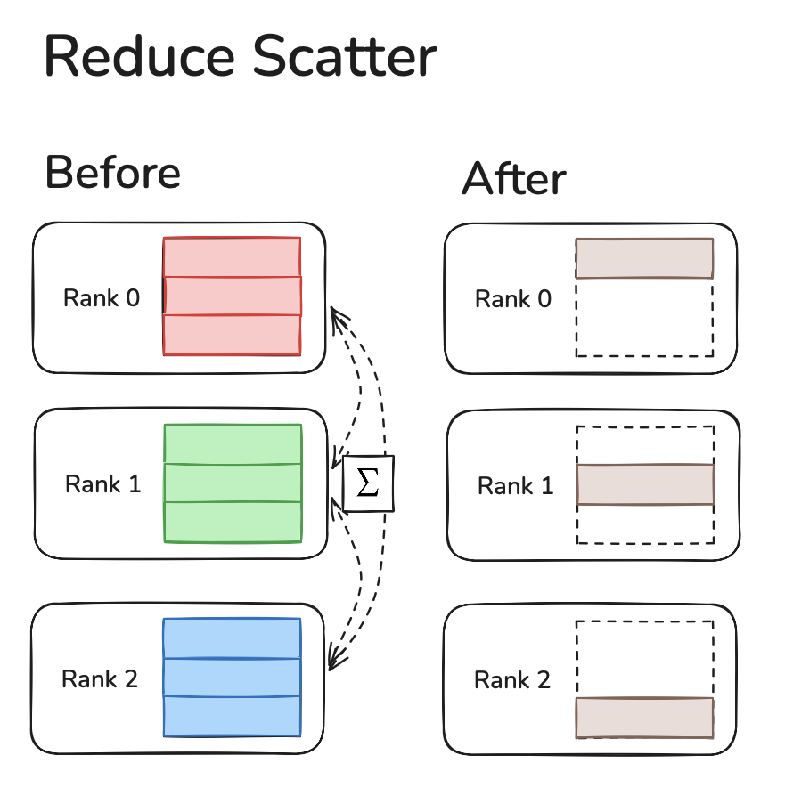
Reduce-Scatter

All Reduce is where data from each device sends all other devices it's data and runs an operation (like SUM, MIN, MAX) to reduce the data.

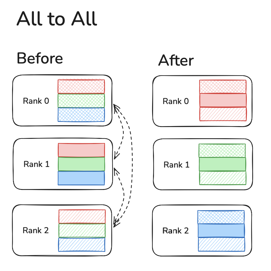
All-to-All

All Reduce is where data from each device sends all other devices it's data and runs an operation (like SUM, MIN, MAX) to reduce the data.

Aside

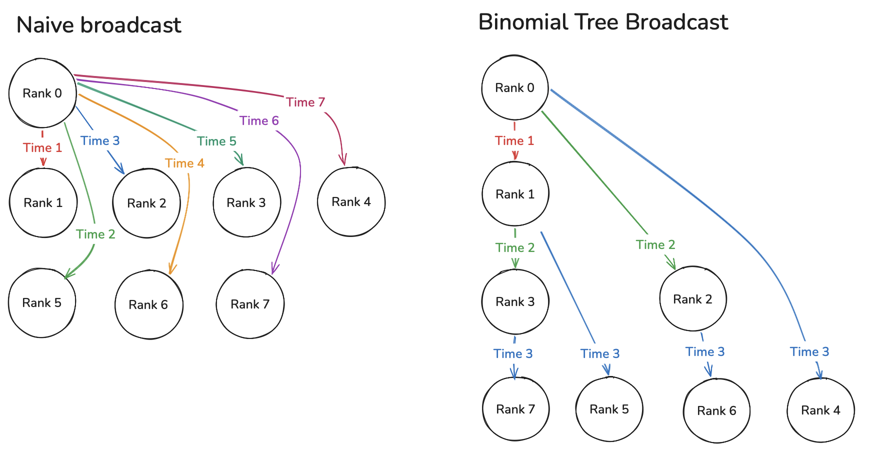
While in theory a broadcast is "parallel", in reality at the hardware level, data is transferred to other devices one device at a time or sequentially with O(N) time complexity. If we view the ranks as a tree as shown below, we can transfer data in O(log(N)) time. The intuition is after rank 0 sends data to rank 1, rank 1 can send data to rank 3 while rank 0 sends data to rank 5, and so on... this pipelining makes it efficient.

Axes of paraLLMelism

I am coining the word parallmelism \s.

mpirun / torchrun are used to run the same program across GPUs. When one runs mpirun mpirun --oversubscribe -np 4 uv run python -m src.model_ddp, mpirun spins up 4 processes and runs model_ddp.py program on each process while assigning each process an id we refer to as rank (0...3).

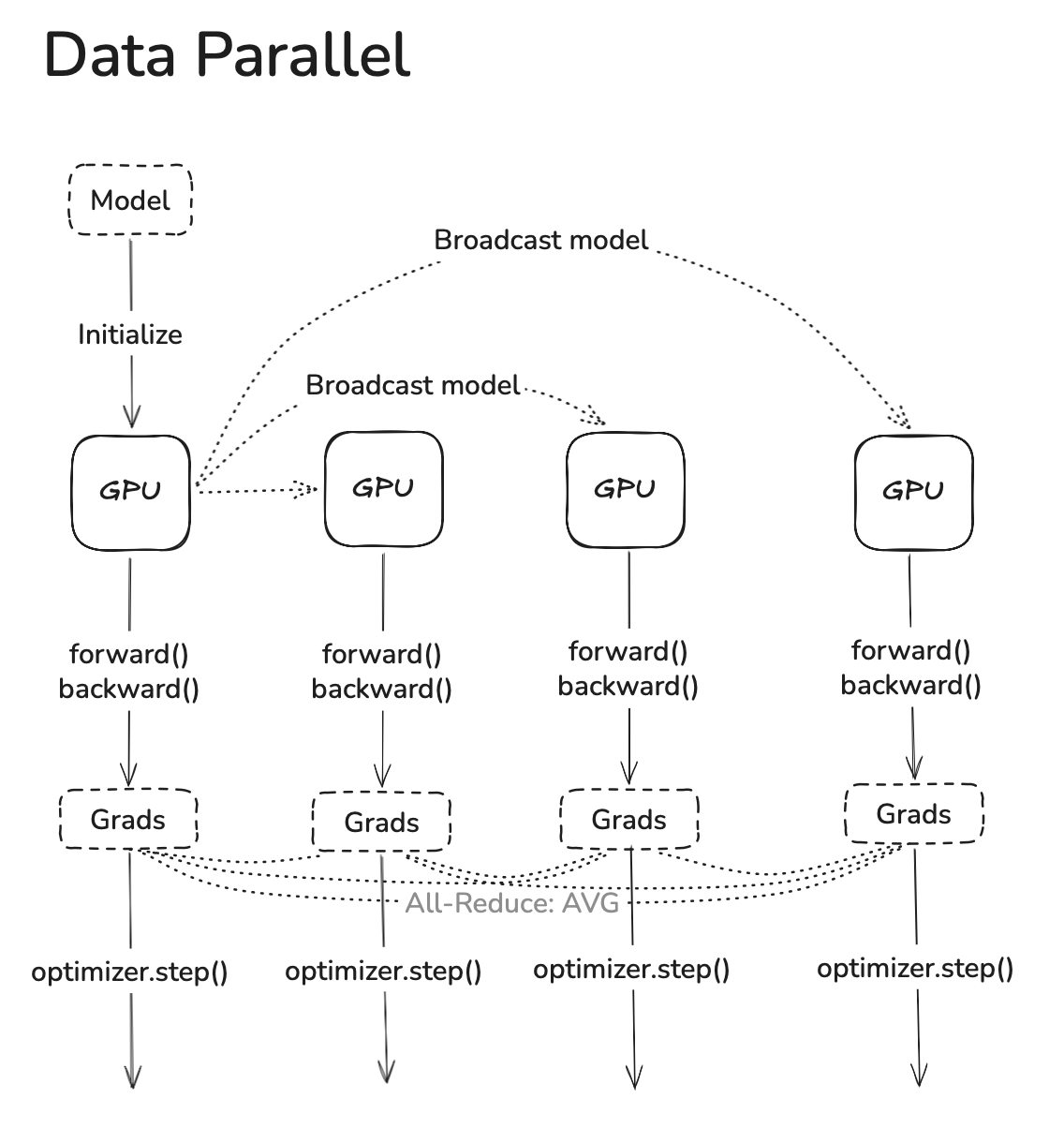
Data parallel

This is the simplest axis to scale on. The same program is run across ranks (using mpi/torch run), when rank0's model is initialized, broadcast it's weights to every other rank to ensure they start with the same weights. Each program's seed should be different so they read different data batches. Then after the forward and backward passes, the gradients should be all-reduced to get the average of all gradients. Since all ranks start off with the same weights and end up with the same average gradient in each step, the optimizer state is same in each step.

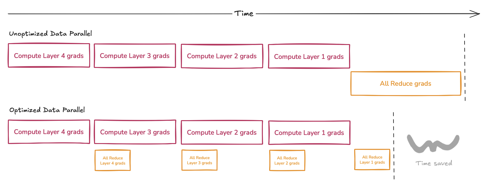
Pytorch has a module called DistributedDataParallel which has some interesting optimizations. For large models, backward passes take on the order of seconds, so it does not make sense to do massive grad reductions once at the end. Therefore, as grads are calculated one by one over the backwards graph, they get added to a bucket and once that bucket reaches > 25MB (6.25M params), we run an async all-reduce. So roughly by the time all grads are calculated, they get all-reduce'd as well.

Pipeline parallel

Pipeline parallelism (PP) is the simplest axis to understand after DP to understand. You simply host chunks of layers on each device.

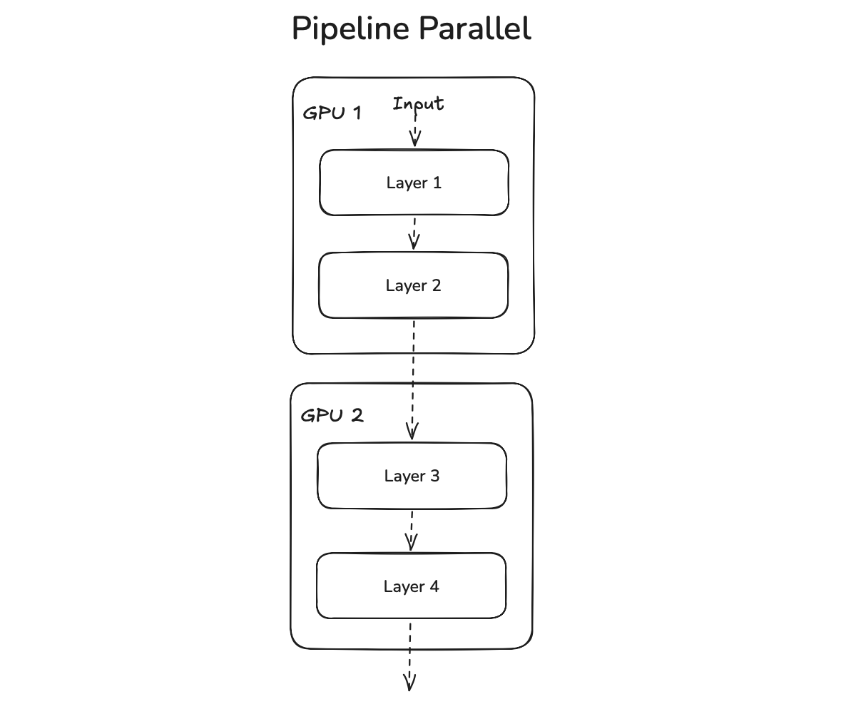
While this is simple, there is one glaring problem at scale. At the 100k GPU scale, communication costs are already high. If one full batch needs to traverse through the forward pass, only the GPU where the currently forwarding layers live will be utilized. This is a perf. engs' and maybe finance team's nightmare.

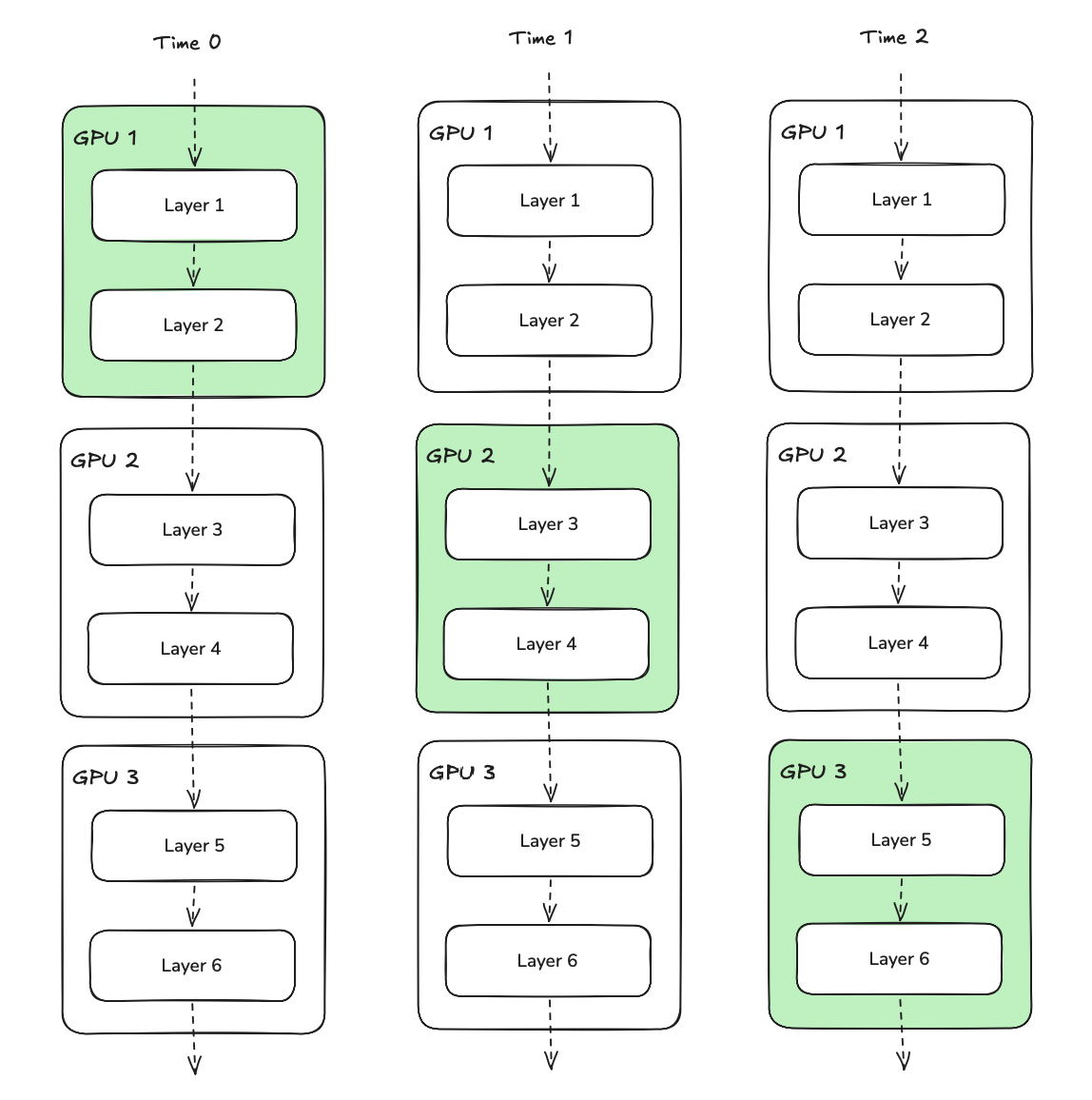
As show above, only one GPU is doing work (in green) at a time, while the others are idle. This idleness of a GPU in the pipeline is called a pipeline bubble. A fix to this is using multiple microbatches for forwards and backwards which reduces the bubble fraction (or # of bubbles in the pipeline).

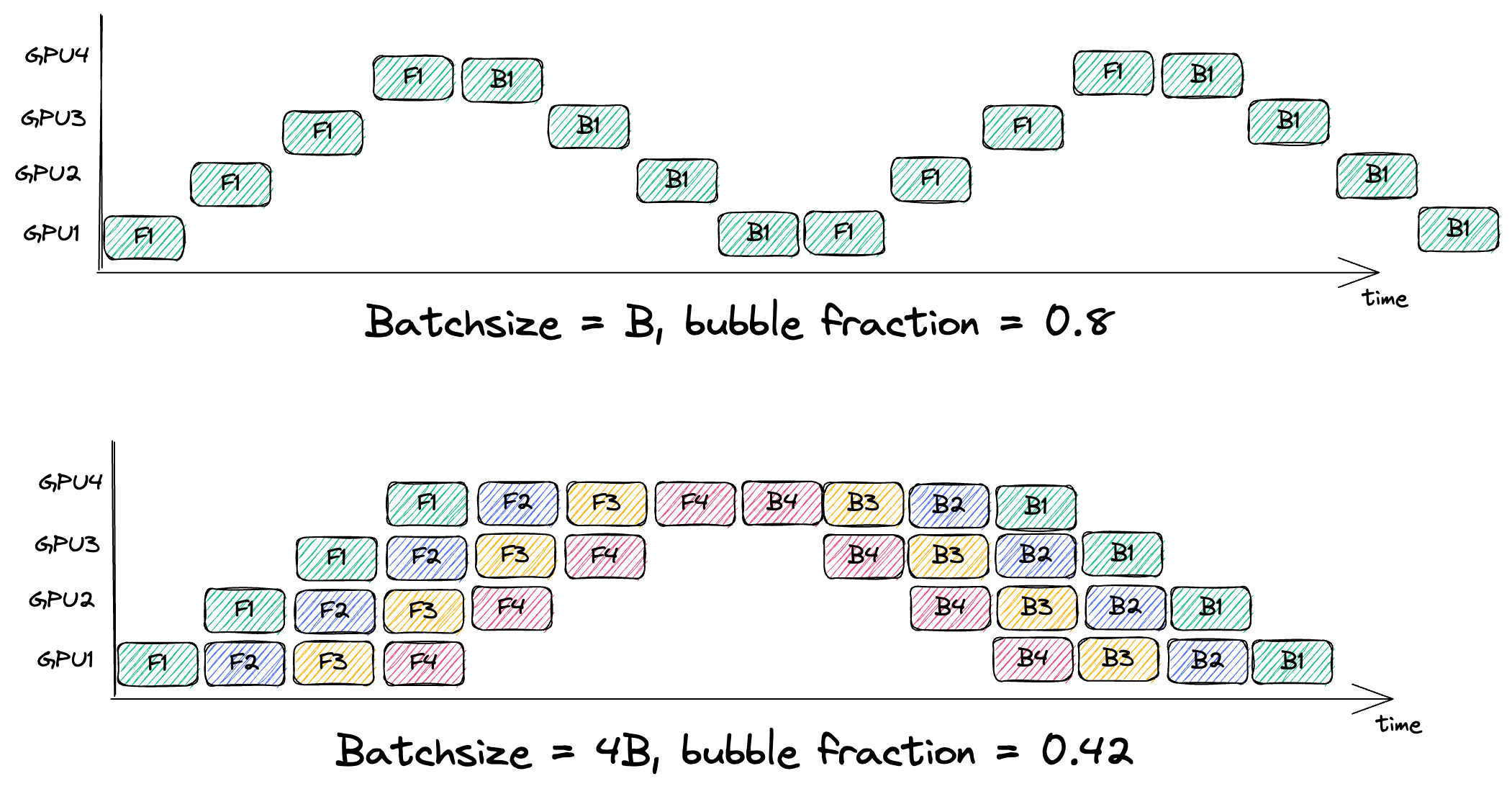
This image is from Simon Boehm's blog on Pipeline Parallelism, I don't think there is a better blog on this. It clearly shows how increasing the microbatches decreases the bubble fraction or empty space relative to total space.

I would go a bit deeper on newer algorithms for this, but 1) I think Simon has covered them really well and 2) I'll keep it for a separate blog.

Tensor parallel

Tensor parallel sounds simple but needs some practice to be easy to intuit. The idea is to horizontally (row-parallel) and/or vertically (column-parallel) split a weight tensor across GPUs. This is usually done on massive Linear layers of FFNs within a transformer.

Take the following example:

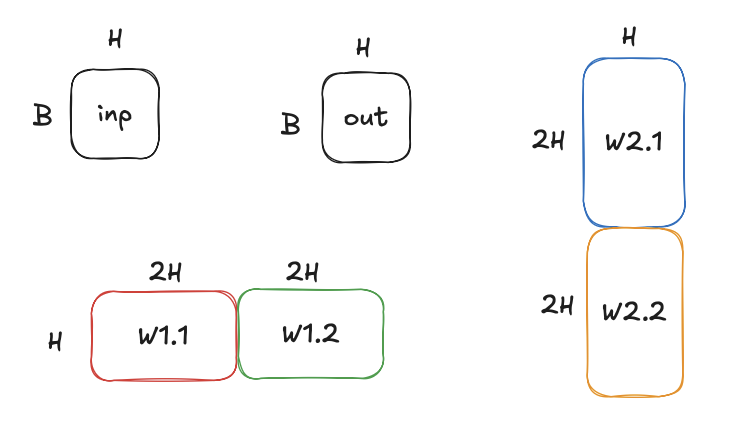
out = W₂(σ(W₁(inp))) where inp has dims [B, H], W₁ is [B, 4H] and W₂ is [4H, B]

These weights get split like below and the WX.1 is assigned to GPU 1 & WX.2 is assigned to GPU 2. This way, we use all GPUs during the compute passes without bubbles.

This is how the FFN will be done.

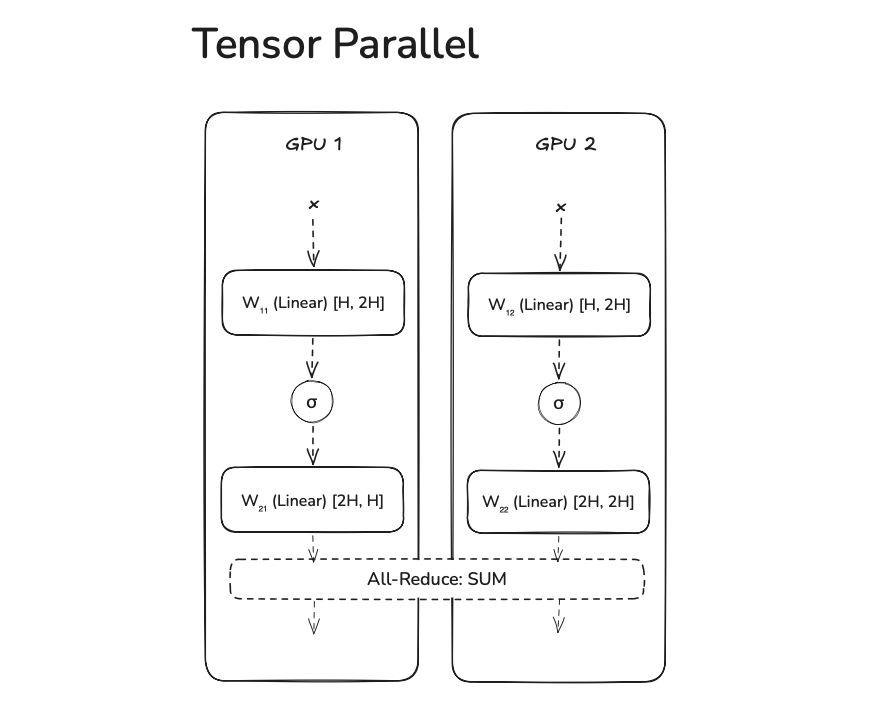
Notice how we avoid all-gathering right after W1 is done on both GPUs, this is because we don't need the fully materialized matrix. Activation functions are element-wise and W_{2, Y} only needs its respective W_{1, Y} chunk. But since the next piece of the compute graph needs the full activation, we need to all-reduce SUM on the partial activations.

Expert parallel

As the name suggests, we put a subset of experts (mixture-of-experts) on each GPU. Nvidia's blog covers this concept well here. This image of theirs demonstrates small- vs large- scale EP.

The concept of expert parallel is simple, implementing it in practice is hard. I guess the biggest challenge with expert parallelism is MoE itself. It takes a lot of surrounding infrastructure like load balancing experts to make sure we don't end up with hot nodes or GPUs where experts are frequently used. Ideally, if we have 4 gpus and 16 experts (4 per gpu), each GPU has one "hot" expert, although this is an active research area.

Early Conclusion

I had a lot more planned for this blog but I realized it's a very redundant topic and there are much better resources that go into more detail. My goal is to write detailed work (usually a documentation of my project written post-work) with illustrative diagrams, but if someone else has done a better job, I'd rather you read that.